(E0 261) Database Management Systems

Sample Questions (Final) - Answers

1. Database Mining

 

1. Yes, my partner's claim is true. Firstly, we have to show that every frequent itemset in the lattice is either itself complete or is a subset of a complete-frequent itemset. That is, the set of complete-frequent itemsets forms a ``cover'' for all frequent itemsets. This proof will ensure that we know the identities of all frequent itemsets.

   Proof: Let ${\cal C}$ be the set of complete-frequent itemsets, for each of which we are also provided the associated supports. Let $f$ be a generic frequent itemset in the lattice. If $f \in {\cal C}$ , then its support is known trivially. Otherwise, let $F$ denote the itemset obtained by the ``round-trip'' operator on $f$ , that is, $F = i (t (f))$ . Now, $F$ has to be a superset of $f$ (because, if $F = f$ , $f$ would be complete, and if $F \subset f$ , the definition of round-trip operator is violated). So, we can be sure that with every incomplete $f$ , there is an associated complete(superset) $F$ . Futher, the associated $F$ has to also be frequent, since its support is exactly equal to that of $f$ , again by the definition of the round-trip operator. Therefore, it will be in ${\cal C}$ . Finally, by the subset-frequency property enumerated in the Apriori paper, every subset of a complete-frequent itemset will also be frequent.

   So, the above shows that ${\cal C}$ is a ``cover'' for ${\cal F}$ , the set of all frequent itemsets.

2. Yes, we can derive the supports of all frequent itemsets from the associated cover, using the following algorithm:

   Do a bottom-up lexicographic traversal of the complete-frequent-itemset lattice - that is, first consider all 1-item complete-frequent itemsets, then all 2-item complete-frequent itemsets, etc. Maintain a dynamic set ${\cal F}$ and for each complete itemset $c$ encountered in the traversal, enumerate all subsets of $c$ and enter those subsets not already in ${\cal F}$ into ${\cal F}$ , along with the associated $c$ .

   At the end of the above traversal, we will have a list of all frequent itemsets along with their associated complete-frequent itemsets. Now the support of each frequent itemset in $f$ in ${\cal F}$ is simply computed as the support of its associated $c$ .

2. Database Warehousing

 

NO, Variance is an algebraic aggregate function.

The variance of a random variable X is defined as $Var(X) = E((X-E(X))^2)$ . This can be re-written as $Var(X) = E(X^2) - (E(X))^2$ .

$E(X)$ and $E(X^2)$ denote $average$ which is an algebraic function, since it can be computed from a 2-tuple consisting of $sum$ and $count$ . Based on the above formula, a 3-tuple $\left\langle sum(X^2), sum(X), count(X)\right\rangle$ is sufficient to compute the variance. Thus a fixed size result can summarize the sub-aggregation implying that the Variance is algebraic.

3. View Selection

 

An easy way to decide the choices is to realize that there is really no point in picking up views $pc$ and $sc$ since their size is exactly the same as $psc$ . So, if we add up the space used by materializing all the remaining views, that comes to less than 7.12M, which is within the bound of 12.5M. Now, neither $pc$ or $sc$ can be (pointlessly) added after this since including them would exceed the 12.5M bound. So, the final choices for materialization are $psc,ps,p,c,s,N$ .

4. View Monotonicity

 

The monotonicity property is that the benefit of any non-selected view monotonically decreases with the selection of other views. That is, $B(V_1, \ldots V_m \mid L) \leq \sum_{i=1}^{i=m} B(V_i \mid L)$ , where $L$ is the original lattice and $V_i$ are the selected views. The monotonicity property is important for the greedy heuristics to deliver competitive solutions. If the optimal solution can be partitioned into disjoint subsets such that the benefit function satisfies the monotonicity property with respect to each of these partitions, then the greedy heuristic guides, at each stage, the selection of an optimal set of views within these partitions.

5. XML Databases

 

A rectangle $(x^1_1, y^1_1, x^1_2, y^1_2)$ contains another rectangle $(x^2_1, y^2_1, x^2_2, y^2_2)$ if the following conditions hold: $C_1: x^1_1 \le x^2_1 \le x^2_2 \le x^1_2$ and $C_2: y^1_1 \le y^2_1 \le y^2_2 \le y^1_2$ . This is similar to the structural join in the Timber paper, where we check if the begin and end of an xml element are contained within the begin and end of another xml element.

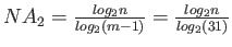
An upper bound can be obtained by building a joint position histogram on all 4 attributes $(X_1, X_2, Y_1, Y_2)$ . Let $H_1$ be the histogram from table $T_1$ and $H_2$ for table $T_2$ and assume that we have $m$ buckets along each dimension. For any tuple in the bucket $(i,j,k,l)$ of $H_2$ , the number of tuples it joins with in $T_1$ is given by $\sum_{i_1\le i, j_1 \ge j, k_1 \le k, l_1 \ge l} {H_1(i_1, j_1, k_1, l_1)}$ . Thus the upper bound is given by $\sum_{i, j, k, l} {H_2(i, j, k, l)*\sum_{i_1\le i, j_1 \ge j, k_1 \le k, l_1 \ge l} {H_1(i_1, j_1, k_1, l_1)}}$ .

6. Main-memory Hash Function

 

1. Using the left-to-right sequence is important in order to maintain the clusters in sorted order which then requires only a ``merge-join'' of the join relation clusters.

2. The reason for settling with radix-based hashing (which is not a particulary good randomizing function) in the paper is that the computation of high-quality randomizing hash functions will itself involve (a) excessive load on the CPU and, more importantly, (b) cause cache misses due to the invocation of the hashing function and its data values.

7. Main-Memory Index

 

L1 cache miss cost $C_1$ = 5 cycles and L2 cache miss cost $C_2$ = 55 cycles.

1. Consider node size to be the L1 cache line size. Thus $c=32, K=4, m=\frac{c}{K}=8$ . Each node access leads to one L1 miss and one L2 miss. Number of nodes accessed, $NA_1 = \frac{log_2n}{log_2(m-1)} = \frac{log_2n}{log_2(7)}$ . The total cost is thus $NA_1*C_1 + NA_1*C_2 = NA_1*(C_1+C_2) = NA_1*60 = \frac{log_2n}{log_2(7)}*60$ cycles.

   Consider node size to be the L2 cache line size. Thus $c=128, K=4, m=\frac{c}{K}=32$ . Each node access leads to four L1 misses (since L1 cache line size is $\frac{1}{4}^{th}$ of 128) and one L2 miss. Number of nodes accessed, $NA_2 = \frac{log_2n}{log_2(m-1)} = \frac{log_2n}{log_2(31)}$ . The total cost is thus $4*NA_2*C_1 + NA_2*C_2 = NA_2*(4*C_1+C_2) = NA_2*75 = \frac{log_2n}{log_2(31)}*75$ cycles.

   It can be seen that it is better to have a node size of 128 bytes.

2. If node size is 32 bytes, number of L1 and L2 cache lines accessed is $(m-1)*2 = 7*2 = 14$ . Thus the total cost is $14*C_1 + 14*C_2 = 14*(C_1+C_2) = 14*60$ cycles.

   If node size is 128 bytes, number of L1 cache lines accessed is $(m-1)*2*4 = 14*4$ and the number of L2 cache lines accessed is $(m-1)*2 = 31*2 = 62$ . Thus the total cost is $14*4*C_1 + 62*C_2 = 56*C_1 + 62*C_2 = 56*5+62*55= 280+3410 = 3690$ cycles.

   It can be seen that the split cost is lower if the node size is 32 bytes.

8. Columnar Databases

 

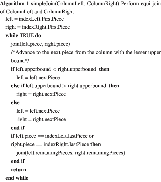
Yes, I agree with the claim. The join algorithm is as follows: